Complete Guide on Deep Learning Architectures, Chapter 1 on ConvNets

Welcome to my guide where I compiled my intuitions, notes and code on deep learning architectures. As a pre-requisite, you only have to know about basics of deep learning: forward pass, backward pass, activations and so on.

My motivation to write this comes from most of the people finding the theory overwhelming and fail to implement the algorithms (I was one of them!). Before every midterm & final I always made sure I understand intuition enough to solve any problem, I studied from wide range of resources to not get overfitted into one’s intuition, tried to put down everything. I hope this guide will be useful to people who take technical interviews or exams or simply is willing to understand.

Convolutional Neural Networks

Convolution: Basic Ideas

Convolution is an operation used to extract features from data. This can be 1D, 2D or 3D. I’ll explain the operation with a solid example, all you need to know now is that the operation is simply takes a matrix made of numbers, moves it through the data, takes the sum of products between the data and that matrix. This matrix is called kernel or filter. You might say, “what does it have to do with the feature extraction and how am I supposed to apply it?”.

Don’t panic! We’re getting to it.

To illustrate the intuition, I’d like us to take a look at this example. We have this 1D data and we visualize it.

I have this kernel [-1, 1]. I’ll start from left-most element, put the kernel, multiply the overlapping numbers and sum them up. Kernels have something centers, it’s one of the elements. Here, we pick the center as 1 (the element on the right). Now, the kernel’s center has to touch every single element, so we put a zero to the the left of the element for convenience. If I don’t pad it, I’ll have to start multiplying -1 with the left-most element, and 1 will not touch the left-most element, that’s why we apply padding. Let’s see how it looks like.

I’m multiplying the left-most element (that is currently a pad) with -1, the first element (zero) with 1 and sum them up, get a 0 and note it down. Now, I’ll move kernel by one position and do the same, note it down again, this movement is called striding, this is usually done by moving the kernel by one pixel, you can also move it with more pixels. The result (convolved data) is currently an array [0, 0].

I will repeat it until the right element of kernel touches every element, which yields the below result.

Notice anything? The filter gives changes in the data (the derivatives!), this is one characteristic we could extract from our data. Let’s visualize.

The convolved data (result of the convolution) is actually called feature map and it makes so much sense, as it shows, well, the features we can extract, the characteristics related to data, the change.

This is exactly the deal with edge detection filters as well! Let’s see it in 2-dimensional data. This time, our kernel will be different, it will be a 3x3 kernel (could’ve been 2x2 as well, just saying).

This filter is actually quite famous but I won’t spoil it for you now :). Previous filter was [-1 1] meanwhile this one is [-1 0 1], it’s just 3x3 and nothing different, it gives changes on the horizontal axis as well. Let’s see an example and apply convolution. Below is our 2D data.

Think of this as an image and we want to extract the horizontal changes. Now, the center of the filter has to touch every single pixel, so we pad the image.

The feature map will be the same size as the original data. The result of the convolution will be written to the same position that the center of the kernel touched in the original matrix, meaning, for this one, it will touch the left-most and the top position.

If we keep applying the convolution we get following feature map.

Which shows us the horizontal change, the edges. This filter is actually called the Prewitt Filter.

You can flip the Prewitt filter to get the changes in vertical direction. Sobel filter is another filter for edge detection.

Convolutional Neural Networks

Fine, but what does it have to do with deep learning? Well, brute forcing filters to extract features does not work well with every image. We could somehow find the optimal filters used to extract important information, or even detect objects in the images. That’s where convolutional neural networks come into play. We convolve images with various filters, and these pixels in the feature maps will eventually become our parameters that we will optimize, and in the end, we will find the best filters for our problem.

The idea is, we will use filters to extract information. We will randomly initialize multiple filters, create our feature maps, feed it to a classifier and do back propagation. Before diving into it, I’d like to introduce you to something we call “pooling”.

As you can see above, there are many pixels that show the change in the feature map. To know that there’s an edge, we actually need to see that there’s one change and that’s it. We can actually get the information that there’s a change (an edge, a corner, anything). In the above example, we could’ve gotten only one of the 2’s, and that would be enough. This way, we will store less parameters and still have the features. This operation of getting the most important element in the feature map is called pooling. With pooling, we lose the exact location of a pixel where there’s an edge, but end up storing less parameters. Also, this way, our feature extraction mechanism will be more robust to small changes, e.g. we only need to know that there are two eyes, a nose and a mouth to know that there’s a face in an image, the distance between those elements and the size of those elements tend to change from face to face, and pooling enables the model to be more robust against these changes. Another good thing about pooling is that it helps us handle varying input sizes. I’d like you to watch this video to gather a better intuition. Below is the max pooling operation, where every four pixels, we get the maximum pixel. There are various types of pooling, e.g. average pooling, weighted pooling or L2 pooling.

Let’s get to the architecture. We will use a Keras example and I will walk you through what’s happening. Below is our model (again, don’t panic, I will walk you through what’s happening).

If you don’t know what Keras Sequential API is doing, it stacks layers like lego bricks and connects them. Each layer has different hyperparameters, Conv2D layer takes number of convolution filters, kernel size and activation function, while MaxPooling2D takes pooling size, and dense layer takes number of output units (again, don’t panic).

Most of the convnet implementations don’t do padding for the sake of letting kernel touch every pixel in an image processing fashion, since padding with zeroes come with an assumption that we might have features in borders, and it adds a complexity for calculation on top. That’s why you’re seeing that the first input size is (26,26), we lose information along the borders.

model = keras.Sequential(
    [
        keras.Input(shape=input_shape),
        layers.Conv2D(32, kernel_size=(3, 3), activation="relu"),
        layers.MaxPooling2D(pool_size=(2, 2)),
        layers.Conv2D(64, kernel_size=(3, 3), activation="relu"),
        layers.MaxPooling2D(pool_size=(2, 2)),
        layers.Flatten(),
        layers.Dropout(0.5),
        layers.Dense(num_classes, activation="softmax"),
    ]
)

model.summary()

Model: "sequential"
_________________________________________________________________
Layer (type)                 Output Shape              Param #   
=================================================================
conv2d (Conv2D)              (None, 26, 26, 32)        320       
_________________________________________________________________
max_pooling2d (MaxPooling2D) (None, 13, 13, 32)        0         
_________________________________________________________________
conv2d_1 (Conv2D)            (None, 11, 11, 64)        18496     
_________________________________________________________________
max_pooling2d_1 (MaxPooling2 (None, 5, 5, 64)          0         
_________________________________________________________________
flatten (Flatten)            (None, 1600)              0         
_________________________________________________________________
dropout (Dropout)            (None, 1600)              0         
_________________________________________________________________
dense (Dense)                (None, 10)                16010     
=================================================================
Total params: 34,826
Trainable params: 34,826
Non-trainable params: 0
_________________________________________________________________

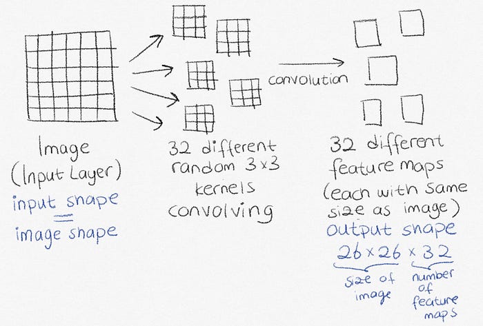
Convolutional neural networks start with an input layer and a convolutional layer. Keras Conv2D layers take number of kernels and the size of the kernel as parameters. What’s happening is illustrated below. Here, we convolve the image with 32 kernels and end up with 32 feature maps, each having the size of the image.

After convolutional layers, we put a max pooling layer to reduce the number of parameters stored and make the model robust to the changes, as discussed above. This will reduce the number of parameters calculated.

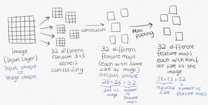
Then, these feature maps are concatenated together and are flattened.

Later on, we use something called dropout to drop a portion of parameters to avoid overfitting. Finally, the final form of weights will go through dense layer for the classification part to finally get classified and backpropagation will take place.

Backpropagation in Convolutional Neural Networks in Theory

How does the backpropagation work here? We want to optimize for the best kernel values here so they’re our weights. At the end, we expect the classifier to figure out relationship between pixel values, kernels, and classes: we have a very long flattened array consisting of elements that consist of pooled and activated version of pixels convolved with initial weights (kernel elements), and we update those weights such that we answer the question “which kernels should I apply to make a distinction between cat and a dog photo?”. So point of training CNNs is to come up with the optimal kernels, and these are found thanks to backpropagation. Prior to CNNs, people would try to try a lot of filters on an image to extract features themselves, meanwhile most generic filters (like we’ve seen above, e.g. Prewitt or Sobel) do not necessarily need to work for all images given images can be very different, even in the same dataset. This is why CNNs outperform traditional image processing techniques.

There are couple of advantages by means of storage when we use convolutional neural networks.

Parameter sharing

In convolutional neural networks, we convolve with the same filter across all pixels and all images which provides an advantage over storing parameters, this is much more efficient than going through an image with a dense neural network. This is called “weight tying” and those weights are called “tied weights”. This is also seen in autoencoders.

Sparse Interactions

In densely connected neural networks, we input the whole piece of data at once -which is very overwhelming due to how images have hundreds or thousands of pixels-, meanwhile in convnets, we have smaller kernels that we use to extract features. This is called sparse interaction, and it helps us use less memory.